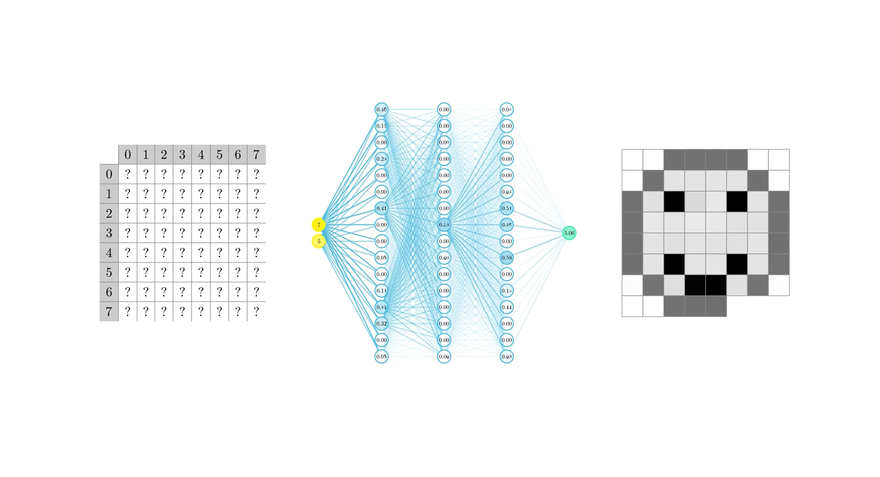
Implicit Neural Representations: A New Way to Remember
Discover how Implicit Neural Representations are revolutionizing data storage and interpretation. This blog post gives a fresh perspective on mimicking human memory through continuous functions, showcasing breakthroughs in data compression, interpolation, and data interpretabilityPublished on 3/20/2025
12 min read
How do We Remember
Technology has long been developed to mimic the natural world. However, computing sets itself apart in this matter with its rigorous structure. For example, data storage is traditionally highly structured, conforming to a list or a grid of bytes. Humans, on the other hand, retain memories as groups of interconnected neurons called ensembles1. Essentially, a knowledge graph about a situation or topic is captured through a network of neurons, which are frequently activated at the same time. To retrieve this information, brain requires a “cue”, which reactivates the same chain2. For example, when forgetting a person’s name, one might try to think of when they first met, triggering a memory of learning their name. Mnemonics like this act as cues, which trigger a sequence of strongly connected neurons to “find” the memory3.
The approach of storing info as a graph of neuron connections creates strong semantic value for our memories. Similar to database indexes, we retain memories such that we can effectively query a data point, but at the same time don’t have to recall more than we need and can selectively store almost our entire life worth of experiences quite compactly.
Traditionally, structured digital data is stored explicitly. For instance, an image is represented as a 2D grid of pixels:
Here, each value in the image array corresponds to a pixel color. Explicit representations are rather intuitive, but they lack any semantic context, and therefore take up large amounts of space and don’t consider pattern in data.
Another way to store a dataset is implicitly. Instead of storing the data directly, we store a function that generates the data. This is very similar to SVG (Scalable Vector Graphics) files, which store images as a series of mathematical functions (lines, curves, etc.) that can be “rasterized” into pixel values. However, while SVGs require data to already be in a vector format, implicit representations can be learned from any discrete data.
To do so, we must learn some function that maps some property of the data to the data itself. Traditionally, data point coordinate is used for this mapping:
Here, , which takes a position as input and outputs the pixel color at that position. Now, in order to save or transmit this image, we only need the function . Additionally, we can interpolate between data points, discover trends, and even interpret the data in novel ways.
Neural Networks as Implicit Representations
Generating a function that represents a dataset is a non-trivial task, and this is where neural networks come in. Neural networks (specifically the Multilayer Perceptrons) are universal function approximators, meaning they can represent almost any nonlinear function given enough input-output examples. By training a neural network on coordinates and dataset values, we can learn its implicit neural representation.
In this example, the INR has 2 inputs (for each 2D pixel coordinate) and one output. However, the number of network inputs/outputs can be arbitrary. For example, we can represent a color image with 3 outputs, each encoding one of RGB color channels.
To evaluate the quality of an Implicit Neural Representation, we need to find how similar reconstructed data is to the original. Traditionally, we use metrics like PSNR (Peak signal-to-noise ratio) and SSIM (Structural similarity index measure). PSNR is essentially (omitting a few aspects of the formula) the inverse of normalized mean squared error, where is no similarity at all and is a perfect match. However, PSNR only takes global error into account, such that a reconstruction can look noisy, but still have high PSNR. This is why we pair it with SSIM, which considers relative luminance, contrast, and structure and approximates perceived quality difference. When training a neural network, we can introduce these metrics as parts of the loss function.
As mentioned in the beginning of this blog post, our goal is to pursue benefits of biological memory networks. However, it is important to note that biological neurons have very little in common with mathematical neurons in how they function. You can read more about here: https://doi.org/10.3390/biology12101330.
Data Compression
One of the key uses of implicit representations is data compression. Since we can often represent high-dimensional data with fewer neurons than data points, this creates an opportunity for data compression. The compression is lossy (reconstructed data will never perfectly recreate the original), but modern neural networks can achieve high degrees of similarity.
Compared to traditional (computational) methods of lossy compression, INRs rely on detecting trends in data, and therefore can capture them much better in reconstruction.
For instance, here I compressed 3D simulation of Hurricane Isabel4 with an Implicit Neural Representation based on SIREN network5 and a computational compressor TTHRESH6:
With a similar compression ratio of over 20,000x, computation compressor TTHRESH has many visual defects, which is represented by SSIM. Implicit Neural Representation SIREN, however, replicated most of the trends contained within data. When compressing a 4-dimensional dataset, which contains 20 time steps of simulation, results are as follow:
| Original | SIREN INR | TTHRESH | |
|---|---|---|---|
| Size on disk | 1716 MB | 79 KB | 82 KB |
| Compression ratio | 1 | 22182 | 21358 |
| PSNR | 36.49 | 33.00 | |
| SSIM | 1 | 0.96 | 0.90 |
When training a traditional classifier or generative model, overfitting on training data is an absolute evil and should be avoided at all costs. However, since compressive INRs need to recall training data and don’t need to generalize trends, high overfitting is actually the goal.
Interpolation and Neural Rendering
Great advantage of INRs is that they map discrete data on a continuous function. This means that we can query between data points to interpolate data. This is useful for not just increasing resolution of media, but even for generating novel views and projections. For example, NeRF (Neural Radiance Fields) is an INR, which is trained on pictures of an 3D object from different camera positions. The same network is then queried at other camera positions to convert a series of pictures into a 3D model7:
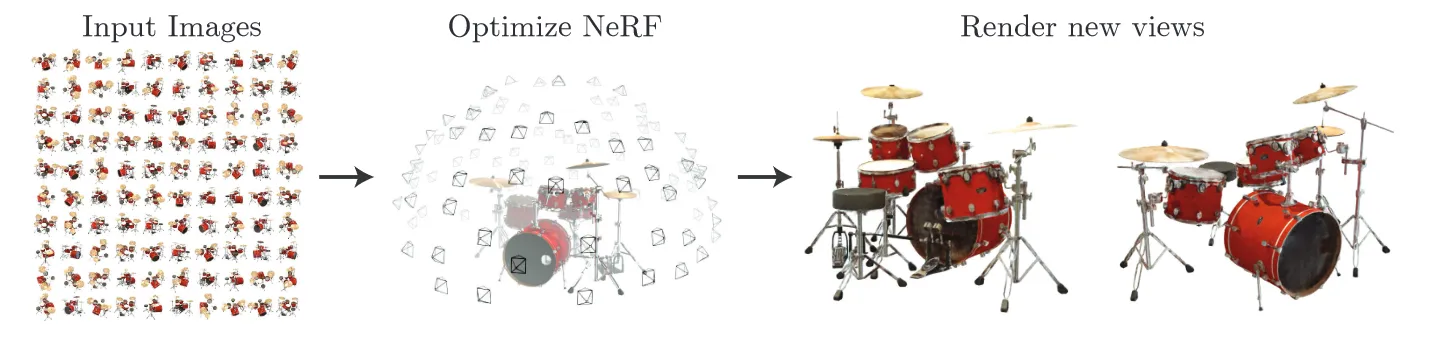
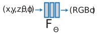
There are 5 inputs to a NeRF model despite working with 3D models. 3 of them represent coordinates of the camera. The other 2 are and angles of the camera direction relative to the object. The output of the model is RGB color of a pixel, and volume density (transparency of a pixel). Frames that NeRF generates are an example of Neural Rendering - generation of frames of known object through Neural Networks.
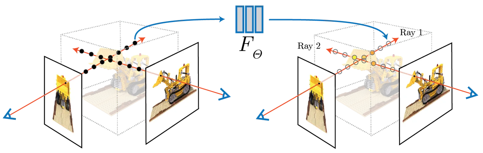
Another interesting feature of NeRF is positional encoding. Since mapping high-frequency spatial coordinates to complex visual scenes is challenging for MLPs, encoding input with more scalars improves model precision. This is similar to when one describes a location in a city to someone, and gives multiple ways to get there, which help identify the location more precisely.
Since camera position and direction are independently parameterized, NeRF can even model change of one independently from other. For example, here we have fixed camera viewpoint, while viewing direction varies:
This method has uses ranging from medical imaging, to computer graphics, to even generating novel views of historical sites.
Trend Analysis and Data Interpretability
Since INRs are mapping discrete data onto a continuous function through finding patterns, we can reverse engineer the learned weights of the network to discover these patterns. This is useful for trend analysis, as we can interpret the data in novel ways. By analyzing the weights of the network, we can discover trends in the data, such as periodicity, trends, and even anomalies.
For example, iHyperTime introduced an INR that evaluates and generates time series data (any data mapped to time, such as weather, financial trends, or social metrics)8. To do, it uses 3 models for different levels of frequency: Trend (polynomial function), Seasonality (learnable Fourier series), and Residual (SIREN INR). This architecture is called TSNet and allows to model and interpret complex time series data with high accuracy.
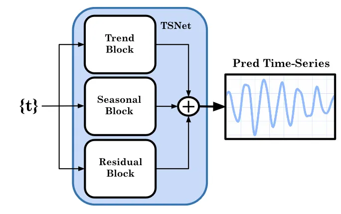
After training a TSNet INR on known data, iHyperTime, uses it to generate new, synthetic time series. It does this with a “hypernetwork” - a network that predicts the parameters (or weights) of TSNet for different time series. Essentially, iHyperTime first summarizes a real time series to capture its trend, seasonality, and residual components, and, by tweaking them, it can generate brand new time series that still look like real data.
For example, here is the distribution and overlap of stock market data generated by iHyperTime and some non-INR models:
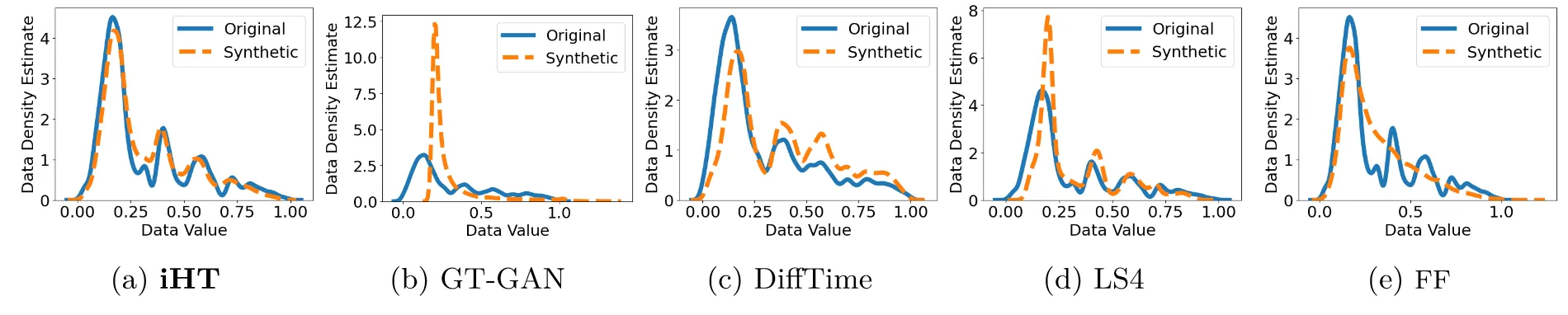
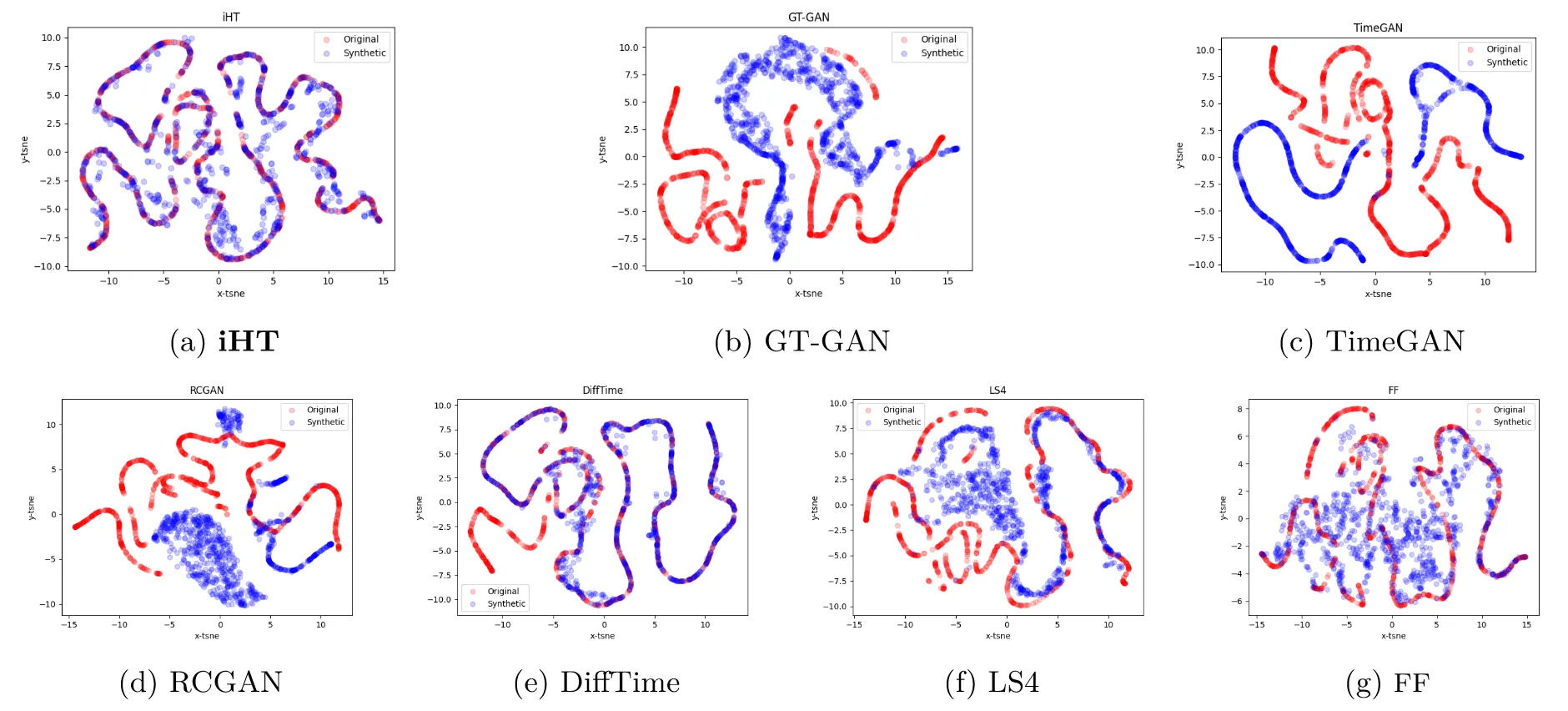
Accurate recreation of data distribution makes iHyperTime a powerful tool for generating quality synthetic data, which can be used for training models, testing algorithms, and even generating novel data for research.
Conclusion and Future Work
Implicit Neural Representations are the closest we have come to mimicking the way human brain stores and retrieves memories, focusing on benefits of semantic implicit memory. They are a powerful tool for data compression, interpolation, and trend detection. Open questions remain on how to improve interpretability of INRs, as well as how to make them more efficient and accurate. However, the potential of INRs is vast, and they are likely to become a new staple in data science and machine learning.
Footnotes
Colom R, Karama S, Jung RE, Haier RJ. Human intelligence and brain networks. Dialogues Clin Neurosci. 2010;12(4):489-501. https://doi.org/10.31887/DCNS.2010.12.4/rcolom. PMID: 21319494; PMCID: PMC3181994. ↩
Frankland PW, Josselyn SA, Köhler S. The neurobiological foundation of memory retrieval. Nat Neurosci. 2019 Oct;22(10):1576-1585. https://doi.org/10.1038/s41593-019-0493-1. Epub 2019 Sep 24. PMID: 31551594; PMCID: PMC6903648. ↩
Wheeler RL, Gabbert F. Using Self-Generated Cues to Facilitate Recall: A Narrative Review. Front Psychol. 2017 Oct 27;8:1830. https://doi.org/10.3389/fpsyg.2017.01830. PMID: 29163254; PMCID: PMC5664228. ↩
Hurricane Isabel data produced by the Weather Research and Forecast (WRF) model, courtesy of NCAR and the U.S. National Science Foundation (NSF). http://vis.computer.org/vis2004contest/data.html/ ↩
Vincent Sitzmann and Julien N. P. Martel and Alexander W. Bergman and David B. Lindell and Gordon Wetzstein. Implicit Neural Representations with Periodic Activation Functions. 2020. https://arxiv.org/abs/2006.09661. ↩
R. Ballester-Ripoll, P. Lindstrom and R. Pajarola, “TTHRESH: Tensor Compression for Multidimensional Visual Data,” in IEEE Transactions on Visualization and Computer Graphics, vol. 26, no. 9, pp. 2891-2903, 1 Sept. 2020, doi: 10.1109/TVCG.2019.2904063. https://doi.org/10.1109/TVCG.2019.2904063 ↩
Ben Mildenhall and Pratul P. Srinivasan and Matthew Tancik and Jonathan T. Barron and Ravi Ramamoorthi and Ren Ng. NeRF: Representing Scenes as Neural Radiance Fields for View Synthesis. 2020. https://www.matthewtancik.com/nerf ↩ ↩2 ↩3 ↩4
iHyperTime: Interpretable Time Series Generation with Implicit Neural Representations. Elizabeth Fons and Alejandro Sztrajman and Yousef El-Laham and Andrea Coletta and Alexandros Iosifidis and Svitlana Vyetrenko. Transactions on Machine Learning Research. 2024. https://openreview.net/forum?id=GSnGPgeoS5 ↩ ↩2 ↩3 ↩4